Colorectal Cancer Risk Prediction

Batch normalization and imputation were used during preprocessing to account for variability and missing values. In metabolomics, data is usually collected in batches through liquid chromatography-mass spectrometry (LC-MS). Since each batch may introduce variability, dividing each batch by the median for a particular metabolite makes the batches more comparable. Null data entries were replaced with the minimum observed metabolite value across all batches.

A major obstacle was that the dataset contained information on the concentrations of 1,224 different metabolites from only 84 patient samples, meaning dimensionality was very high relative to sample size. In addition to the concentrations of different metabolites in each participant's stool sample, clinical data such as age, sex, FIT, and Cologuard results were also provided. FIT detects hidden blood in stool, while Cologuard combines this with DNA analysis for mutations or epigenetic markers from precancerous polyps.

One of the first control models we developed aimed to predict CRC risk using only metabolite data and achieved a test accuracy of around 58%. Since SVMs use a kernel to implicitly project data into a higher-dimensional feature space, a dataset of 1,224 metabolites was highly prone to overfitting. I applied dimensionality reduction techniques such as principal component analysis (PCA) and five-fold cross-validation in an attempt to improve performance. However, the model consistently reported a much higher validation accuracy, which indicated that other metrics should be introduced to corroborate the existing metabolomic data.

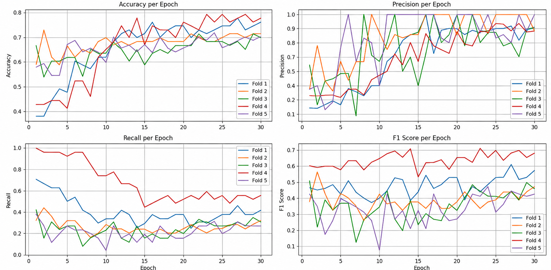
The layered architecture of a neural network was well suited to our goal of creating a single predictive framework for diverse data types. In our model, we used an Adam optimizer to adjust gradients and learning rates for each parameter and a ReLU activation function to capture more complex, nonlinear relationships between variables. I also applied regularization techniques such as dropout and L2 regularization to prevent overreliance on specific neurons and overfitting to noise. After running ten independent cycles with five-fold cross-validation, we achieved an average accuracy of around 59.3%, while integrating clinical data increased this result to 63%.

To incorporate the four new features into the neural network, several adjustments were made to the preprocessing pipeline and model structure. The categorical features were first converted into binary vectors using one-hot encoding, after which both age and metabolomic data were standardized. Interestingly, age and FIT alone yielded the highest accuracy of 72%, which made it clear that noise from using all 1,224 metabolites was overpowering the cleaner signal from the clinical data. As a result, it became necessary to select a smaller number of informative metabolites and evaluate them separately.

The first method we attempted involved univariate feature selection through an ANOVA F-test, which evaluated each metabolite independently against CRC risk. The top twenty metabolites were then used in our MLP neural network and yielded an accuracy roughly equivalent to the previous result. We then determined that recursive feature elimination (RFE) might be more effective, as bootstrapping and subsampling would give a fuller picture of the interactions between metabolites when predicting CRC risk.

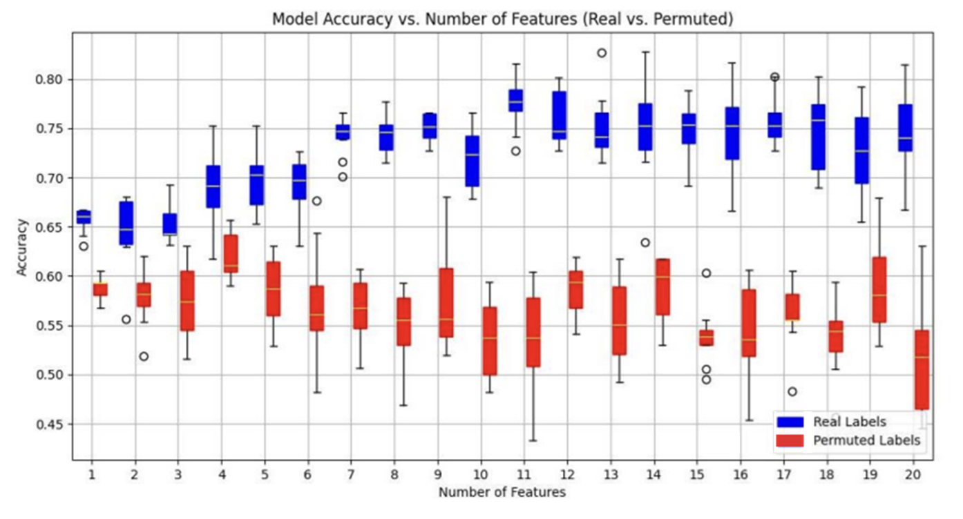
For our final model, since twenty was a relatively arbitrary starting number, I ran RFE with different numbers of metabolites and determined that performance peaked at around ten features, with an accuracy of 80.4%. Using more than ten increased the risk of overfitting and feature redundancy, especially because many metabolites are biologically correlated.

It was also noted early in the project that there was a meaningful class imbalance in the dataset, with low-risk samples (N = 48) outnumbering high-risk samples (N = 33). Three additional confirmed CRC samples were excluded because they would provide limited value for risk-classification training. I then applied SMOTE in an attempt to balance the training-data distribution. However, because this technique generates synthetic samples for a minority group by interpolating between existing samples, it was prone to amplifying the existing noise in our high-dimensional dataset.

These uncertainties made it necessary to use permutation testing to confirm that the observed accuracy reflected real relationships. By randomly assigning risk labels to data points, we found that the distribution of accuracies from permuted labels was consistently lower than that of the real labels, with minimal overlap across varying numbers of top metabolites. Additionally, at ten features, the difference in performance was statistically significant. The box-and-whisker plots below are slightly staggered.

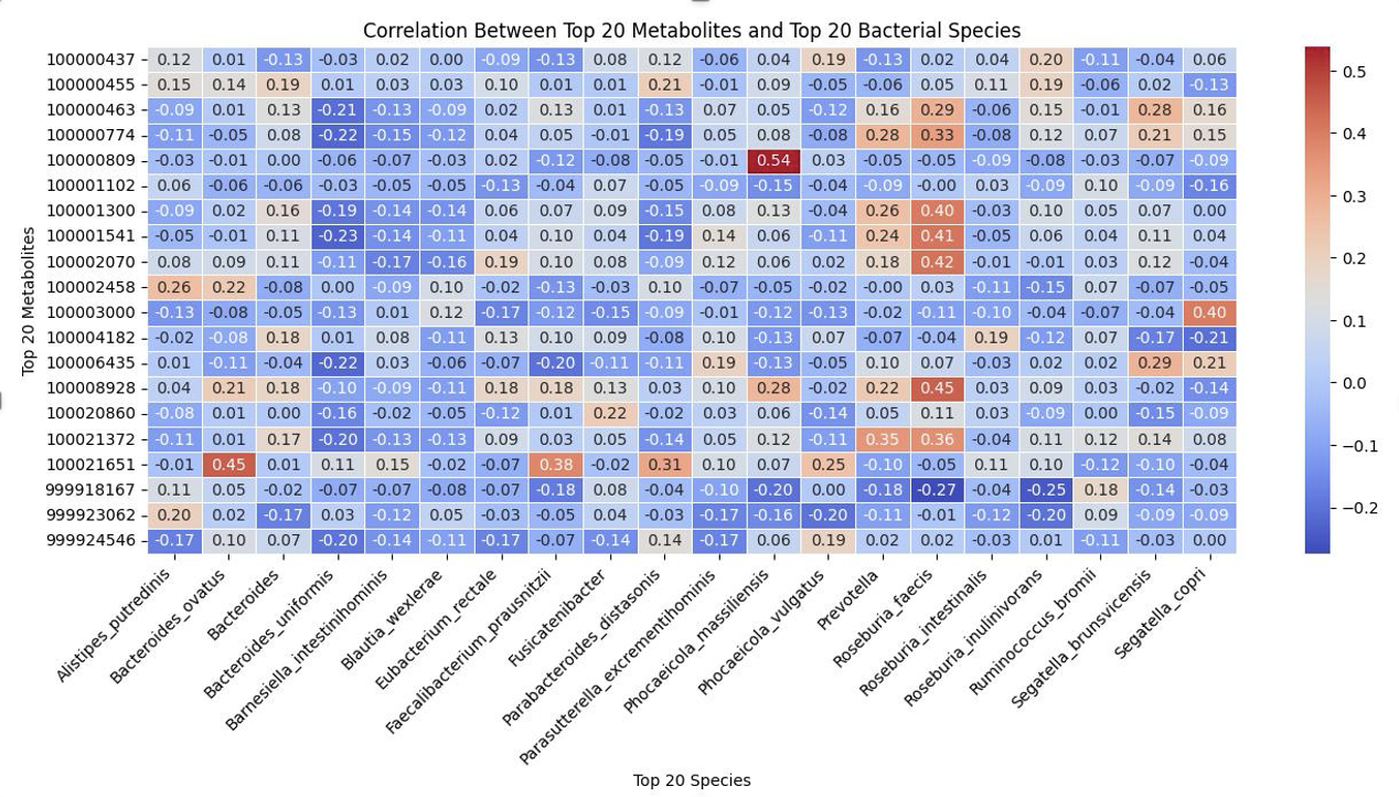
The same process was carried out using data on the concentrations of bacterial species in the samples. Summaries of my literature reviews can be found for both the top bacterial species and the top metabolites. Notable biomarkers include Bacteroides species, indolelactate (ILA), and secondary bile acids.

The last task I was involved with at the Dey Lab was analyzing sequencing data using the existing model framework. FASTQ files stored both the raw DNA sequences obtained from stool samples and their corresponding quality scores. I then used k-mer frequency analysis to process the files and found that k = 6 yielded optimal results. In a biological context, this value may better capture codon information. To normalize the data, the relative frequency of each k-mer was used. Applying RFE again to select the most informative subsequences resulted in an accuracy of 75% using sequencing data alone.

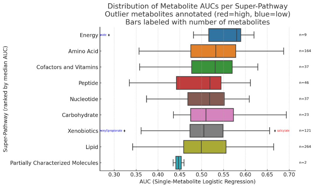
Finally, I computed the area under the curve (AUC) for the ROC curve of each metabolite and grouped the results by biological subpathway, such as fatty acid metabolism and the TCA cycle, and by superpathway, such as amino acids, lipids, and peptides. Work is still being done to visualize patterns in k-mer frequency distributions across samples and integrate sequencing data and pathway analysis into the final model. However, the initial findings demonstrate the potential of this approach. Pathway-level predictive performance could benefit significantly from regularization so that bias from larger pathways does not dominate the results.